Analysis of Railroad Track Defects

Introduction

Condition monitoring and predictive maintenance have become increasingly important in the railway industry, where operational safety and cost efficiency are critical. Failures in track infrastructure pose severe safety risks and result in economic consequences through service interruptions and repair costs. Traditionally, track condition is assessed through scheduled manual inspections or specialized measurement trains. While effective, these methods are costly, time-consuming, and limited in inspection frequency and scope.

One parameter of particular importance is the cant (tilt) of the track, which influences ride comfort, safety, and wear on trains and infrastructure. Inertial Measurement Units (IMUs) mounted on in-service trains can provide continuous data on vehicle dynamics, transforming monitoring from discrete inspections to continuous, data-driven surveillance of track geometry.

This report investigates the use of IMU acceleration data to estimate track cant through a simplified physical model of train-track interaction. The model is validated by comparing simulated accelerations with measured data in the time and frequency domains. The Fast Fourier Transform (FFT) is applied to residuals to identify systematic discrepancies between the model and reality.

Methods

Model

The two forces of interest are centripetal, or lateral, acceleration, $a_c$, and vertical gravitational acceleration, $a_g$. Centripetal acceleration is:

$a_c = \frac{v^2}{r}$

where $v$ is train velocity and $r$ is the radius of curvature. The effect of gravity on a banked curve depends on the cant angle, so measured acceleration can be modeled as:

$a = \frac{v^2}{r}\cos\theta - g\sin\theta$

Model Validation Using FFT

The difference between simulated and measured data is the residual, the part of the measured signal that the model could not explain. If the model captures the system dynamics, residuals should resemble white noise with a flat spectrum. Peaks in the residual spectrum indicate systematic components that the model has failed to capture.

Data

The measured and simulated acceleration data was provided by CEMIT Digital, a company located in Porsgrunn specializing in predictive maintenance and monitoring solutions for the railroad industry.

Implementation

The implementation computes a single-sided amplitude spectrum. It keeps positive frequencies, normalizes magnitudes by $n$, doubles them to account for discarded negative frequencies, and corrects the DC and Nyquist components.

# Sampling rate (Hz)
fs = 500
n = len(ameas)
t = np.arange(n) / fs
xf = fftfreq(n, 1 / fs)[:n // 2]

# FFT calculations
yf_meas = fft(ameas)
yf_sim = fft(asim)
yf_diff = fft(diff)

# FFT processing
yf_abs = np.abs(yf_diff[:n // 2])
yf_diff_proc = (2.0 / n) * yf_abs
yf_diff_proc[0] /= 2
if n % 2 == 0:
	yf_diff_proc[-1] /= 2

Results

Time-Domain Analysis

The simulated model captures the overall trend of the measured acceleration, but its amplitudes are significantly lower. The residual signal closely resembles the measured signal, making clear patterns difficult to distinguish.

Frequency-Domain Analysis

The FFT shows a prominent spike at 0 Hz, likely representing a DC offset caused by the model consistently underestimating or overestimating measured acceleration. Distinct peaks around 3 Hz and 37 Hz appear in both measured and residual spectra. The 3 Hz component may correspond to periodic track features or recurring vehicle dynamics, while the 37 Hz component likely reflects localized or transient phenomena.

Time-Frequency Analysis

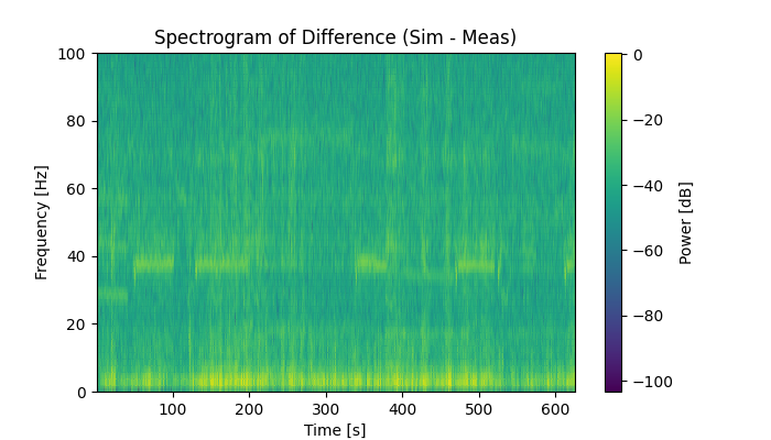
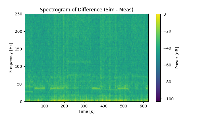
The 3 Hz component appears relatively constant, suggesting a stable track or vehicle characteristic. The 37 Hz component exhibits intermittent on-off behavior, indicating transient events or sections of track with localized irregularities.

Discussion

The amplitude mismatch may arise from inaccuracies in radius of curvature, train velocity, or cant angle. It may also result from unmodeled dynamics including track irregularities, suspension effects, or sensor noise. Because the simplified model accounts only for centripetal and gravitational forces, it may miss important transient and high-frequency effects.

The residual spectrum does not resemble white noise, confirming that the model fails to capture the full dynamic behavior of the train-track system. Persistent low-frequency components and transient high-frequency components should be investigated as possible indicators of recurring or localized track features.

Conclusion

The simplified cant model captures the general trend of the measured IMU data but does not fully reflect system dynamics. It consistently underestimates measured accelerations, and residual components at approximately 3 Hz and 37 Hz demonstrate that the residuals are not white noise.

The model provides a useful baseline but lacks the fidelity required for reliable condition monitoring. Future work should incorporate suspension response, track irregularities, wheel-rail interaction, and larger datasets across varying track and operational conditions. Hybrid approaches combining physics-based modeling with machine learning may offer improved accuracy.